Visualize architectural stripes

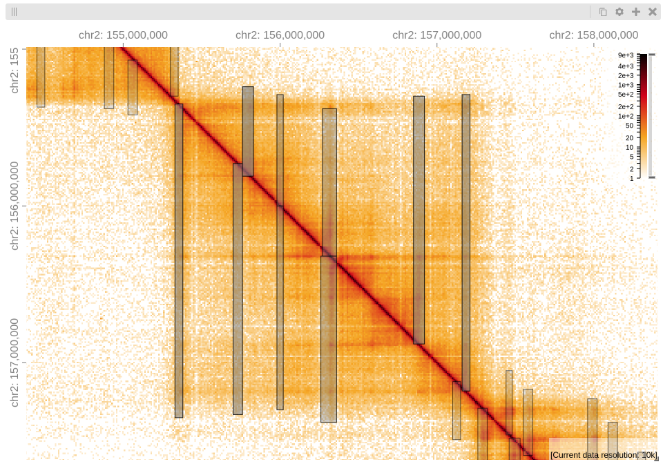
Visually inspecting a subset of the detected stripes is highly recommended to verify that the parameters configured for stripepy call are well-suited to your specific dataset. To assist with this inspection, the Jupyter notebook visualize_stripes_with_highlass.ipynb is provided. This notebook is designed to work with input files in the .mcool format.

If your matrix is in .hic format you can easily convert it to .mcool format using hictk by running hictk convert matrix.hic matrix.mcool. HiGlass cannot visualize single-resolution Cooler files. If you are working with .cool files you can use hictk to generate .mcool files by running hictk zoomify matrix.cool matrix.mcool.

For more details, please refer to hictk’s documentation: hictk.readthedocs.io.

We recommend running the notebook using JupyterLab.

Furthermore, the notebook depends on a few Python packages that can be installed with pip. Please make sure that the following packages are installed in a virtual environment that is accessible from Jupyter. Refer to IPython’s documentation for instructions on how to add a virtual environment to Jupyter.

pip install 'clodius>=0.20,<1' 'hictkpy>=1,<2' 'higlass-python>=1.2,<2'

Next, launch JupyterLab and open notebook visualize_stripes_with_highlass.ipynb.

jupyter lab

Before running the notebook, scroll down to the following cell

mcool = ensure_file_exists("CHANGEME.mcool")
bedpe = ensure_file_exists("CHANGEME.bedpe")

and set the mcool and bedpe variables to the path to the .mcool file used to call stripes and the path to the stripe coordinates extracted with stripepy view, respectively.

mcool = ensure_file_exists("4DNFI9GMP2J8.mcool")
bedpe = ensure_file_exists("stripes.bedpe")

Now you are ready to run all cells.

Running the last cell will display a HiGlass window embedded in the Jupyter notebook (note that the interface may take a while to load).