Quickstart

StripePy is organized into a few subcommands:

• stripepy download: download a minified sample dataset suitable to quickly test StripePy.

• stripepy call: run the stripe detection algorithm and store the identified stripes in a .hdf5 file.

• stripepy view: take the result.hdf5 file generated by stripepy call and extract stripes in BEDPE format.

• stripepy plot: generate various kinds of plots to inspect the stripes identified by stripepy call.

Walkthrough

The following is a synthetic example of a typical run of StripePy. The steps outlined in this section assume that StripePy is running on a UNIX system. Some commands may need a bit of tweaking to run on Windows.

1) Download a sample dataset (optional)

If you need to download the example matrix used here, you can do so by running:

user@dev:/tmp$ stripepy download --name 4DNFI9GMP2J8

Feel free to use your own interaction matrix instead of 4DNFI9GMP2J8.mcool. Please make sure the matrix is in .cool, .mcool, or .hic format.

A more extended description of the subcommand stripepy download is found in Downloading sample datasets.

2) Detect architectural stripes

The stripepy call subcommand is the core of the analysis, designed to identify architectural stripes within contact maps. This process can be quite time-consuming, especially when working with large files.

The path to your contact map file and the desired resolution are required to run the analysis. For instance, to analyse the 4DNFI9GMP2J8.mcool file at a 10,000 bp resolution, you would use:

user@dev:/tmp$ stripepy call 4DNFI9GMP2J8.mcool 10000

The command will output a single HDF5 file (e.g., 4DNFI9GMP2J8.10000.hdf5).

Additional information is provided in Detect architectural stripes.

3) Fetch stripes in BEDPE format

Stripe coordinates can be fetched from the .hdf5 file using stripepy view, as in

user@dev:/tmp$ stripepy view 4DNFI9GMP2J8.10000.hdf5 > stripes.bedpe

Further details can be found in Fetch architectural stripes.

4) Generating plots

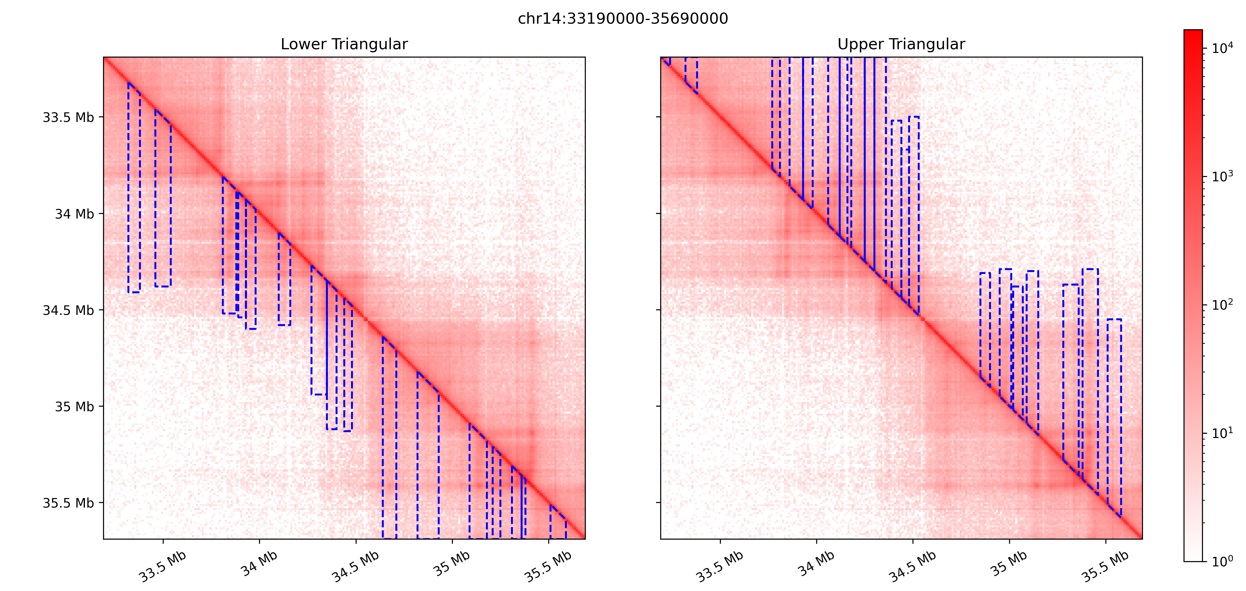
StripePy comes with a plot subcommand that can be used to visualize architectural stripes overlaid on top of the Hi-C matrix. stripepy plot can also generate several graphs showing the general properties of the called stripes, see Generating plots for a complete overview.

For instance, running

user@dev:/tmp$ stripepy plot cm 4DNFI9GMP2J8.mcool 10000 /tmp/matrix_with_stripes.png --stripepy-hdf5 4DNFI9GMP2J8.10000.hdf5 --highlight-stripes

will generate the following plot

Accessing stripes and descriptors from Python

If you are working in Python, you might want to carry out analysis on the stripes and their biodescriptors. The ResultFile class helps load and process HDF5 files (e.g., 4DNFI9GMP2J8.10000.hdf5) generated by StripePy.

The following code snippet can be used to load lower-triangular stripes over the whole genome:

In [1]: from stripepy.data_structures import ResultFile

In [2]:  with ResultFile("4DNFI9GMP2J8.10000.hdf5") as f:
   ...:      df = f.get(
   ...:          chrom="chr1",     # Pass None to fetch data for all chromosomes
   ...:          field="stripes",  # See API docs for a complete list of supported fields
   ...:          location="LT",    # Use "UT" to fetch from the upper-triangle
   ...:      )
   ...:

In [3]: df
Out[3]:
       seed  top_persistence  left_bound  right_bound  top_bound  ...  outer_lmean  outer_rmean  outer_mean  rel_change  cfx_of_variation
0        93         0.398490          91           96         93  ...     0.180769     0.240014    0.210392   19.138436          0.563444
1       102         0.053084          99          105        102  ...     0.250077     0.246783    0.248430    1.276074          0.605748
2       108         0.082636         106          111        108  ...     0.251255     0.242434    0.246845    6.744239          0.629097
3       116         0.103803         114          119        116  ...     0.452872     0.395339    0.424105    3.394272          0.394917
4       130         0.073611         126          132        130  ...     0.235412     0.249025    0.242219    3.656868          0.608349
...     ...              ...         ...          ...        ...  ...          ...          ...         ...         ...               ...
1743  24693         0.057216       24687        24695      24693  ...     0.274141     0.284040    0.279090    5.741370          0.382488
1744  24708         0.048084       24706        24710      24708  ...     0.280574     0.322965    0.301770    7.036960          0.354274
1745  24720         0.044175       24718        24723      24720  ...     0.162981     0.155803    0.159392    5.192390          0.833381
1746  24733         0.054484       24730        24737      24733  ...     0.181836     0.191120    0.186478    0.238297          0.791300
1747  24793         0.052317       24790        24796      24793  ...     0.168377     0.219650    0.194013    7.811918          0.518017

[1748 rows x 22 columns]