Generating plots

It is often a good idea to visually inspect at least some of the stripes to make sure that the used parameters are suitable for the dataset that was given to stripepy call. StripePy comes with a plot subcommand that can be used to generate various kinds of plots.

stripepy plot supports the following subcommands:

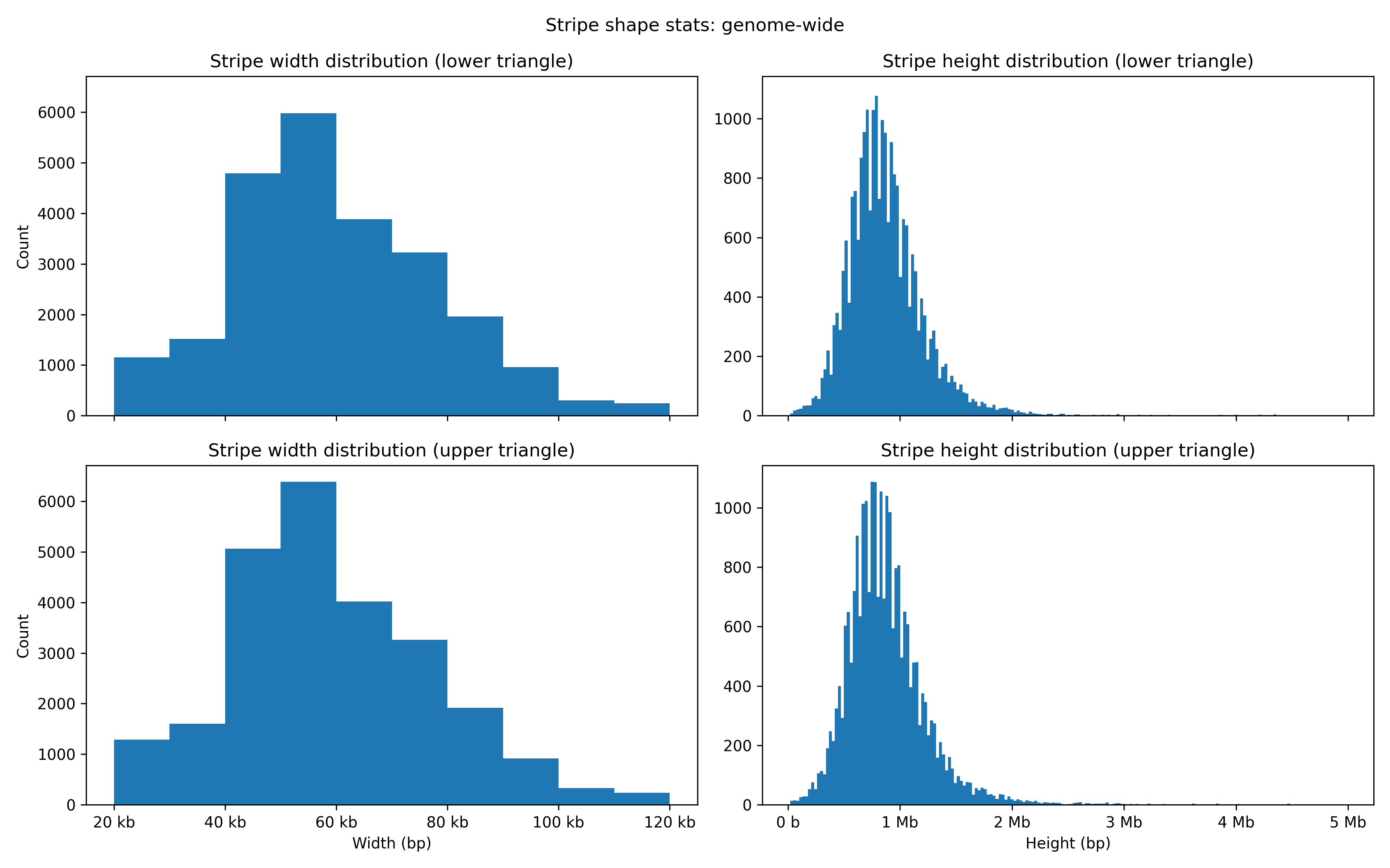
• contact-map (cm): plot stripes and other features over a region of the Hi-C matrix

• pseudodistribution (pd): plot the pseudo-distribution over a genomic interval

• stripe-hist (hist): generate and plot the histograms showing the distribution of the stripe heights and widths

All three subcommands support specifying a region of interest through the --region option. When the commands are run without specifying the region of interest, stripepy plot cm and stripepy plot pd will generate plots for a random 2.5 Mbp region, while stripepy hist will generate histograms using data from the entire genome.

Plots of contact maps

The stripepy plot cm command can be used to visualize Hi-C contact maps with different levels of annotation. stripepy plot cm takes as input a Hi-C matrix in .cool, .mcool, or .hic format, and optionally the .hdf5 file generated by stripepy call (this parameter is mandatory when highlighting stripes or stripe seeds). We here provide a few examples.

The simplest plot displays the contact map at a given resolution:

# Plot the Hi-C matrix
user@dev:/tmp$ stripepy plot cm 4DNFI9GMP2J8.mcool 10000 /tmp/matrix.png

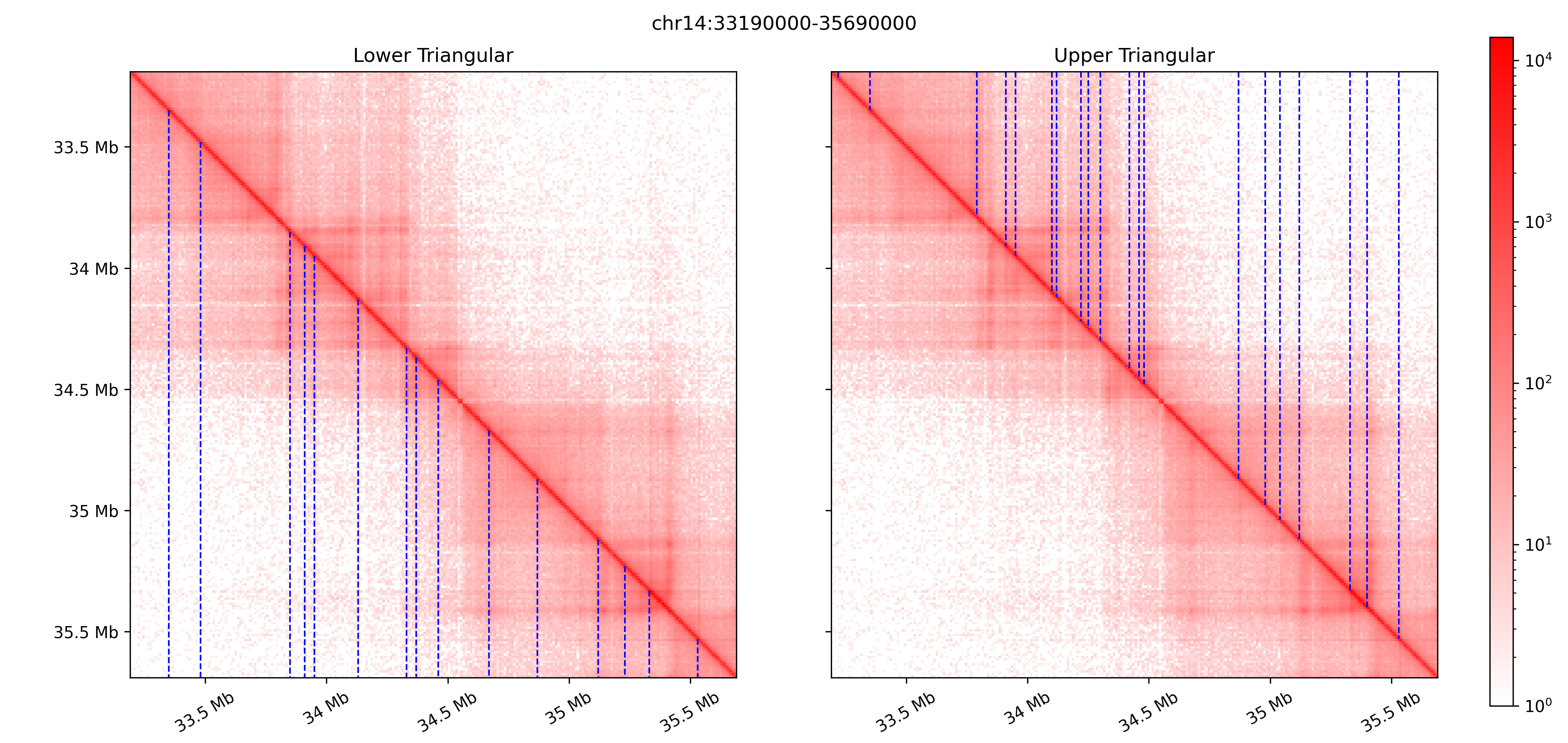
Stripe seeds can be visualized with the option --highlight-seeds. Note that the HDF5 output is required:

# Plot the Hi-C matrix highlighting the stripe seeds
user@dev:/tmp$ stripepy plot cm 4DNFI9GMP2J8.mcool 10000 /tmp/matrix_with_seeds.png --stripepy-hdf5 4DNFI9GMP2J8.10000.hdf5 --highlight-seeds

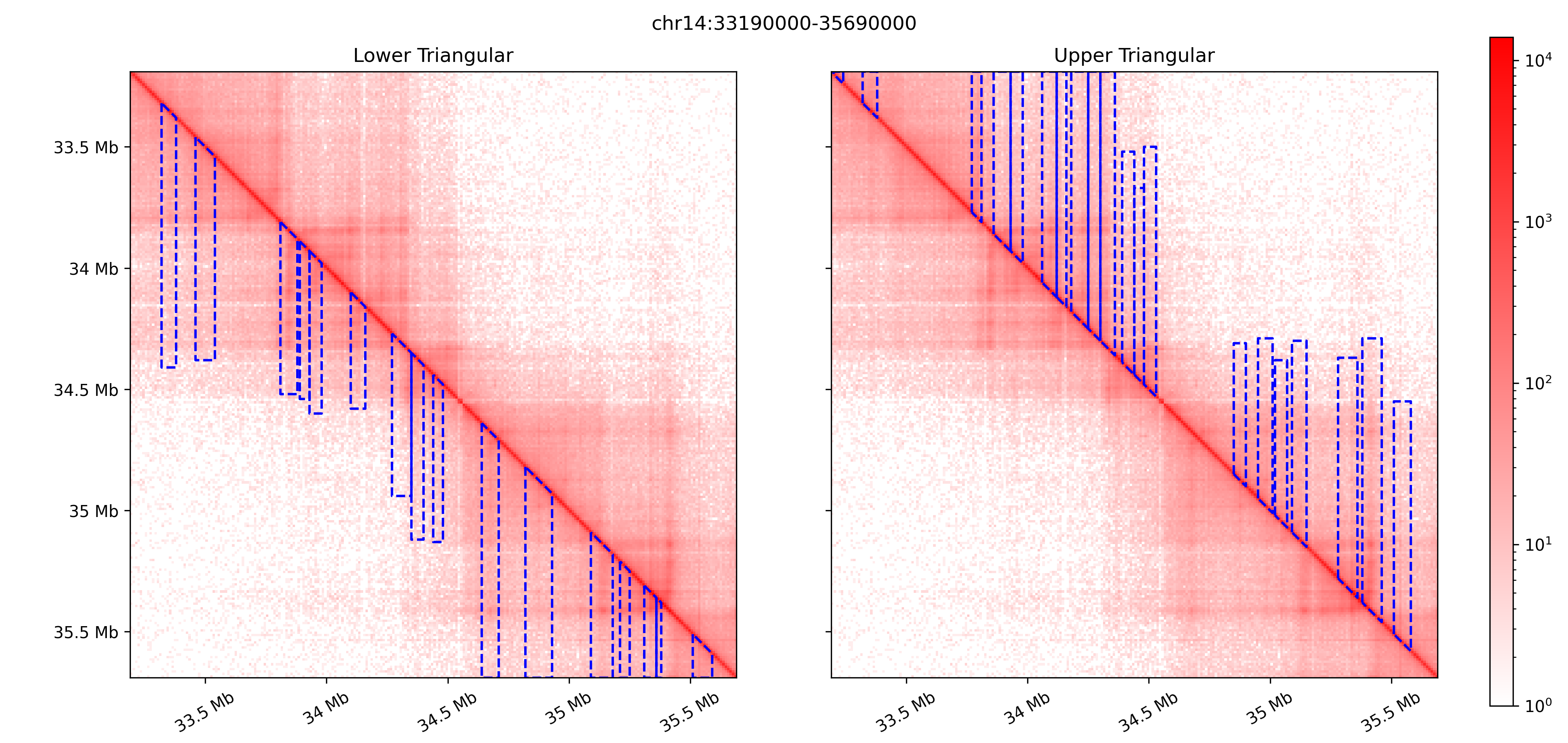
To visualize the detected architectural stripes, use the --highlight-stripes flag. It is possible to visualize the stripes without any thresholding

# Plot the Hi-C matrix highlighting the architectural stripes
user@dev:/tmp$ stripepy plot cm 4DNFI9GMP2J8.mcool 10000 /tmp/matrix_with_stripes.png --stripepy-hdf5 4DNFI9GMP2J8.10000.hdf5 --highlight-stripes

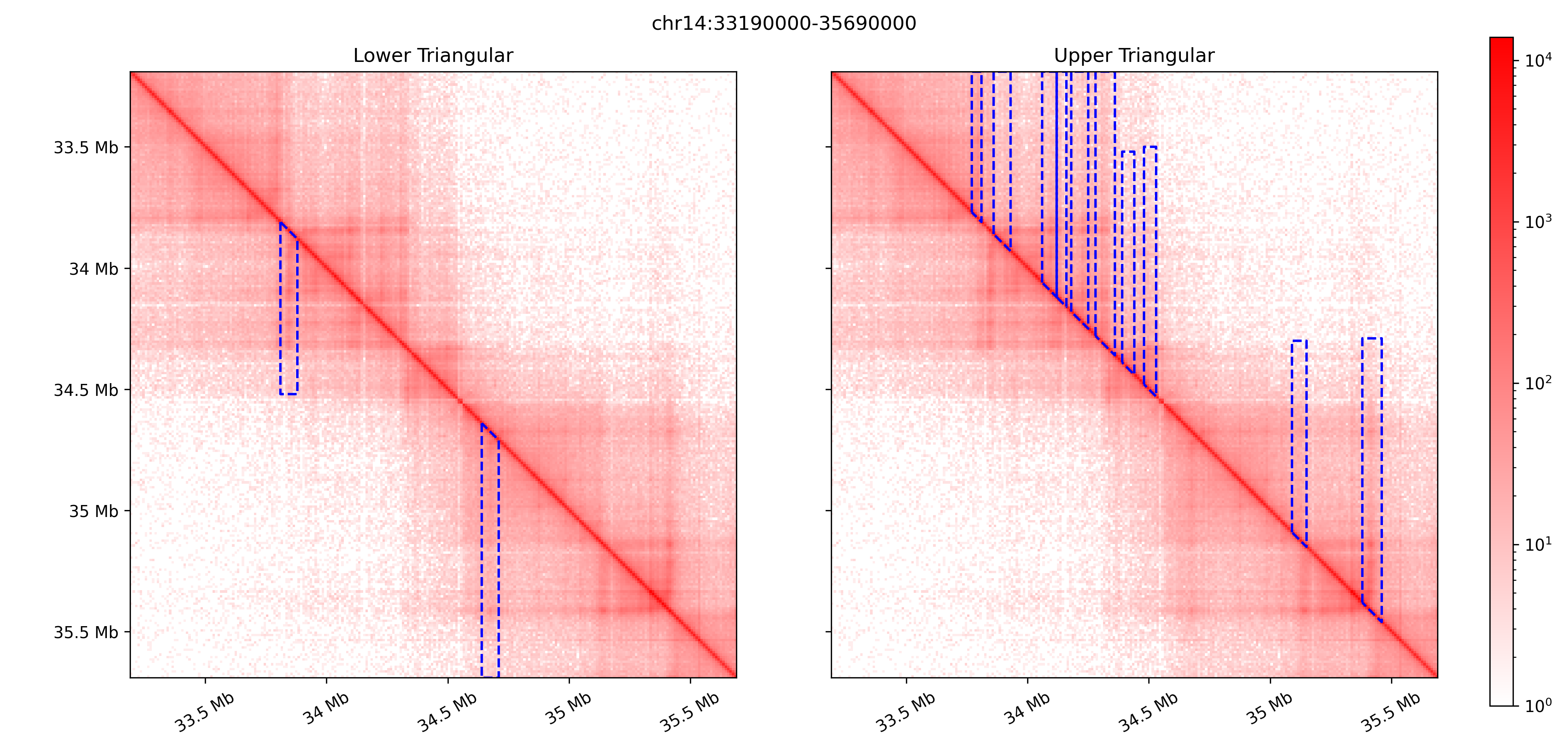
or with thresholding (using either --coefficient-of-variation-threshold, --relative-change-threshold, or both options):

# Plot the Hi-C matrix highlighting the architectural stripes -- thresholding both relative change and coefficient of variation
user@dev:/tmp$ stripepy plot cm 4DNFI9GMP2J8.mcool 10000 /tmp/matrix_with_stripes.png --stripepy-hdf5 4DNFI9GMP2J8.10000.hdf5 --highlight-stripes --coefficient-of-variation-threshold 1 --relative-change-threshold 5

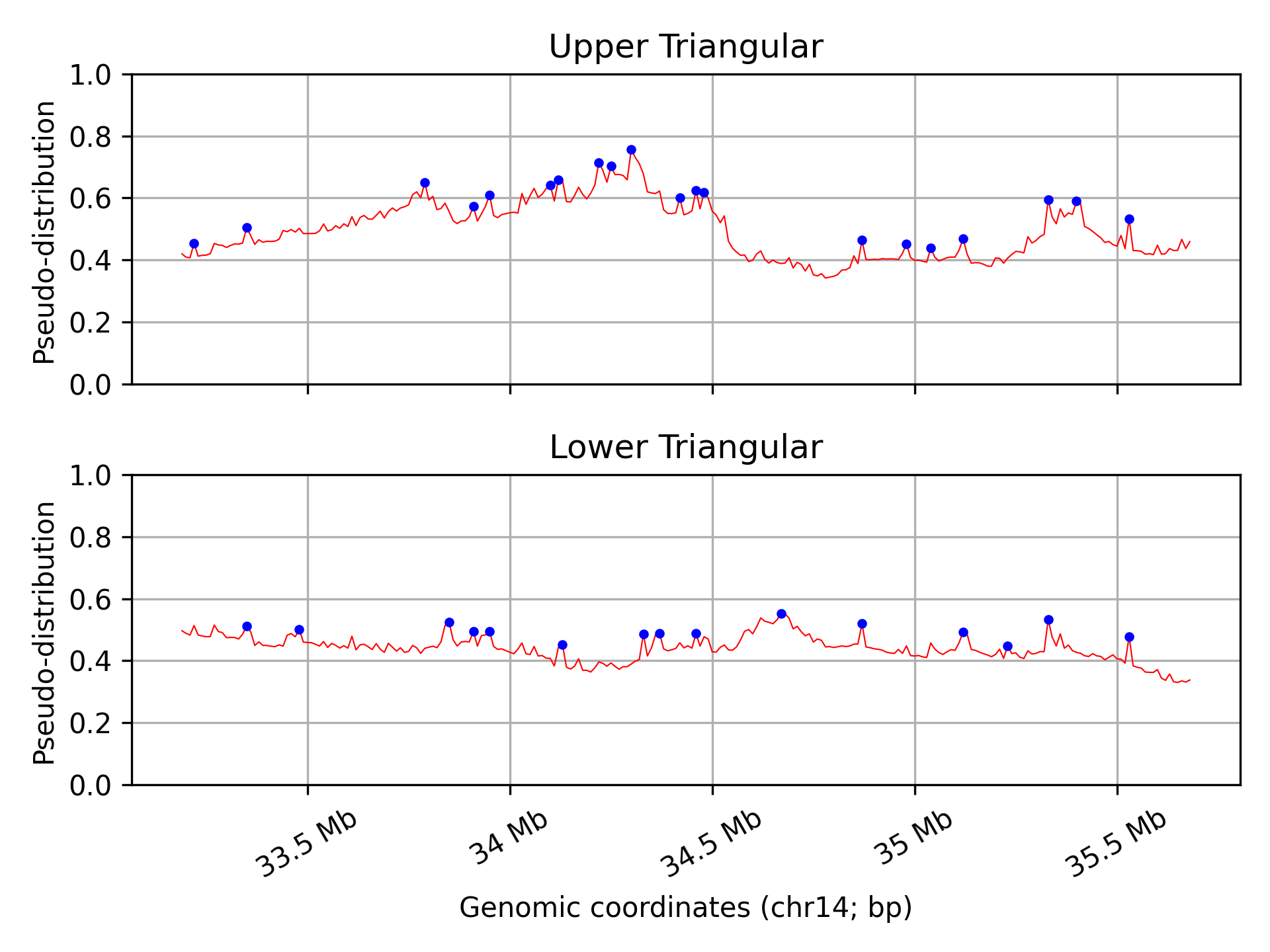
Plots of pseudo-distributions

stripepy plot pd (and stripepy plot hist) does not require the Hi-C matrix file, and require the .hdf5 file generated by stripepy call instead.

Example usage:

# Plot the pseudo-distribution
user@dev:/tmp$ stripepy plot pd 4DNFI9GMP2J8.10000.hdf5 /tmp/pseudodistribution.png

Plots of histograms

stripepy hist uses the .hdf5 file generated by stripepy call to create histograms of .

Example usage:

# Plot the histograms using genome-wide data
user@dev:/tmp$ stripepy plot hist 4DNFI9GMP2J8.10000.hdf5 /tmp/stripe_hist_gw.png

Visualize architectural stripes in HiGlass

We provide a Jupyter notebook visualize_stripes_with_highlass.ipynb to facilitate this visual inspection with HiGlass. The notebook expects the input file to be in .mcool format.

More info available at Visualize architectural stripes with HiGlass.